In the last post, we covered Supervised and Unsupervised Learning briefly. Here, we'll look at Supervised and Unsupervised Learning in detail. There'll will be some maths equation involved but don't worry, we'll break it down as much as possible.

Topics Covered

1. Supervised Learning (Regression, Classification)

2.Unsupervised Learning (k-means and Hierarchical Clustering)

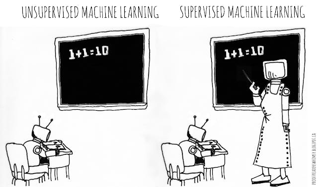
1. Supervised Learning

How much money will we make by spending more dollars on digital advertising? Will this loan applicant pay back the loan or not?

Problems like this are solved using this type of Learning.

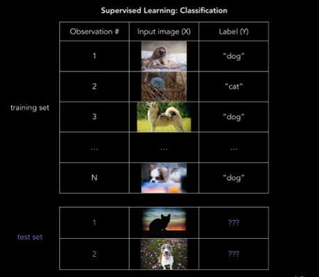
In order to solve these problems, we start with a data set containing training examples with associated correct labels. It's like you show a thousand pictures of cats and dogs to your machine and tell it that it is in fact cats and dogs respectively. The algorithm will then learn the relationship between images and their associated labels (here it is cats and dogs) and apply that learned relationship to classify completely new images (without labels) that your machine hasn't seen before.

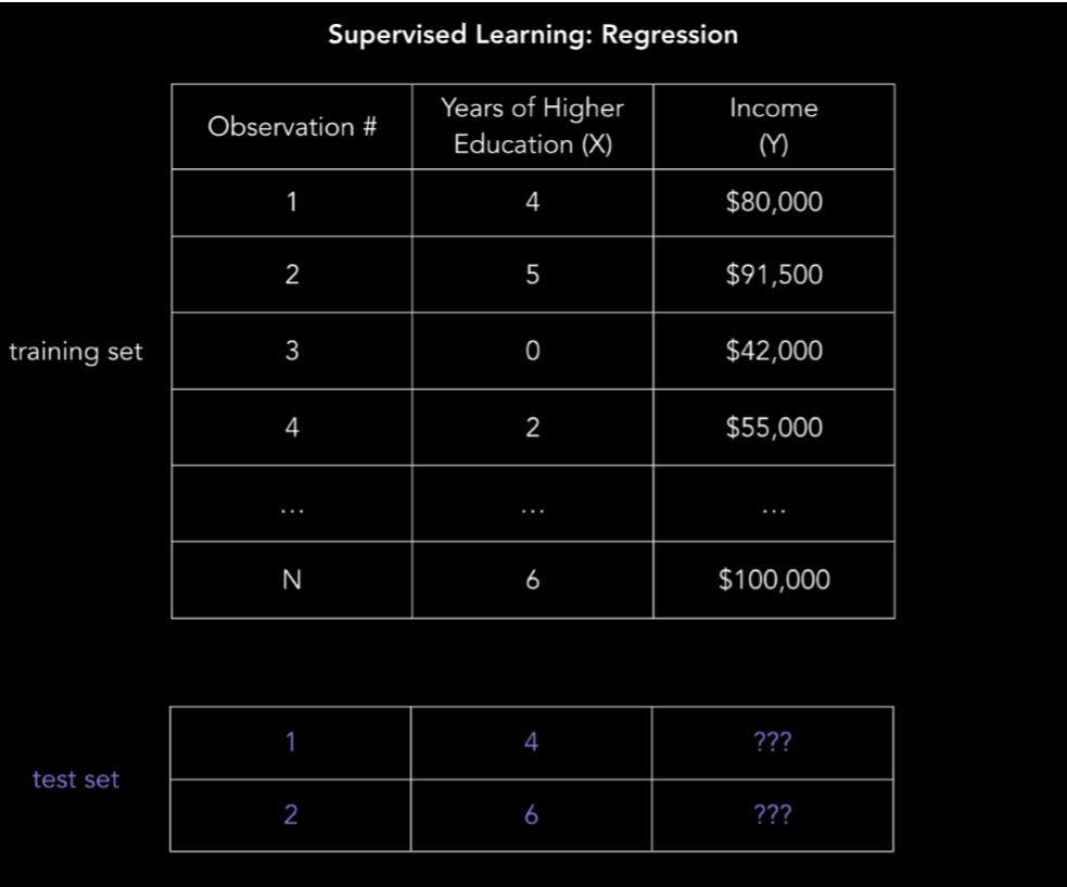
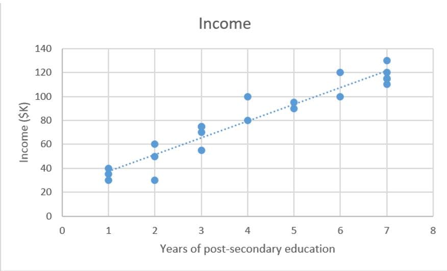
Now we'll see how Supervised Learning works in general. Let's examine the problem of predicting annual income based on the number of years of higher education someone has completed.

Expressed more mathematically, we'd like to build a model that approximates the relationship between f between the number of years of higher education X and corresponding annual income Y.

Y=f(X)+ε

where,

X (input) = years of higher education

Y (output) = annual income

f = function describing the relationship between X and Y

ε (epsilon) = random error term (positive or negative) with mean zero

The machine attempts to learn the relationship between income and education from scratch, by running labelled training data through a learning algorithm. This learned function can be used to estimate the income of people whose income Y is unknown, as long as we have years of education X as inputs. In other words, we can apply our model to the unlabeled test data to estimate Y.

Regression: predicting a continuous value

Regression predicts a continuous target variable Y . It allows you to estimate a value, such as housing prices or human lifespan, based on input data X.

Here, target variable means the unknown variable we care about predicting, and continuous means there aren’t gaps (discontinuities) in the value that Y can take on.

A person’s weight and height are continuous values. Discrete variables, on the other hand, can only take on a finite number of values — for example, the number of kids somebody has is a discrete variable.

     Regression
     Y = f(X) + ε, where X = (x1, x2…xn)
     Training: machine learns f from labeled training data
     Test: machine predicts Y from unlabeled testing data

Coming back to our income prediction example, the data could take the form of a .csv file where each row contains a person's education level and income. Adding more columns with more features will give a more complex, but more accurate model.

Linear Regression (Ordinary Least Squares)

You're going to see some mathematical equations from now on but don't worry about it. The basic idea of Linear Regression is drawing a line, that's it.

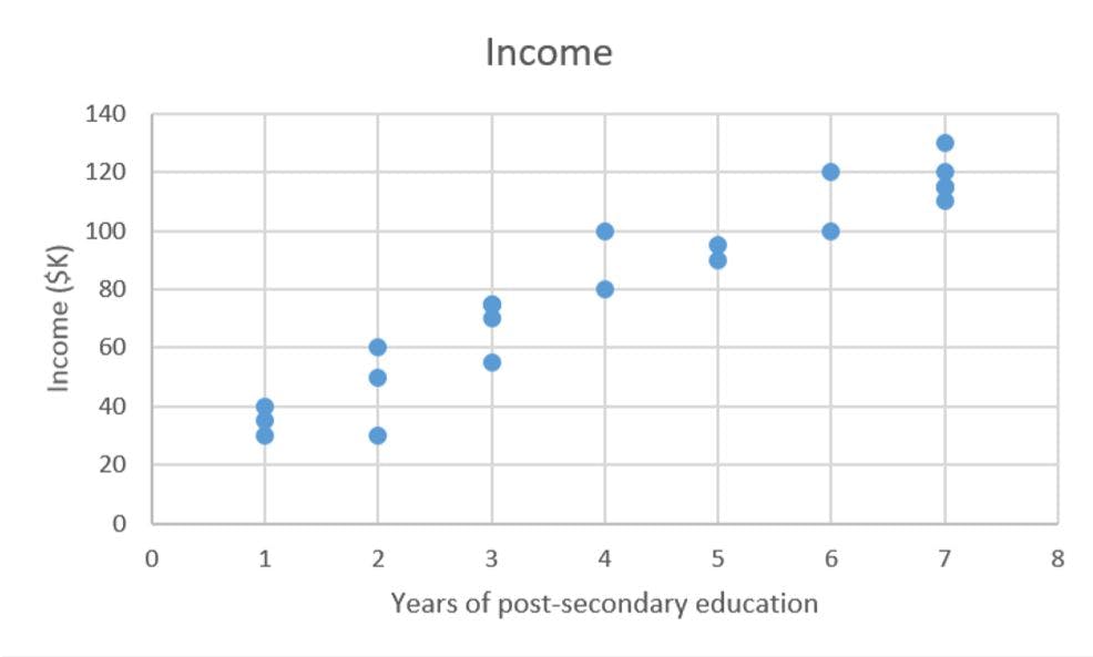
We have our data set X which contains years of post-secondary education and corresponding target values Y which contains corresponding annual incomes . The goal of ordinary least squares (OLS) regression is to learn a linear model that we can use to predict a new y given a previously unseen x with as little error as possible.

   X_train = [4, 5, 0, 2, …, 6] # years of post-secondary education
   Y_train = [80, 91.5, 42, 55, …, 100] # corresponding annual incomes, in thousands of dollar.

Linear regression is a parametric method, which means it makes an assumption about the form of the function relating X and Y. Our model will be a function that predicts ŷ given a specific x:

ŷ=β0+ β1*x+ ε

Our goal is to learn the model parameters (in this case, β0 and β1) that minimize error in the model’s predictions.

Here are the two ways to find the best parameters:

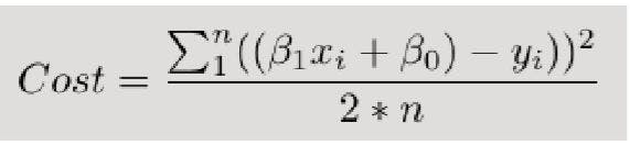
1. Define a cost function, or loss function, that measures how inaccurate our model's predictions are.

2. Find the parameters that minimize loss, i.e make our model as accurate as possible.

Graphically, in two dimensions, this results in a line of best fit as shown below.

Mathematically, we look at the difference between each real data point (y) and our model’s prediction (ŷ). Square these differences to avoid negative numbers and penalize larger differences, and then add them up and take the average. This is a measure of how well our data fits the line.

Everything is fine as long as the cost function is simple. When the cost function is not simple, we have to use an iterative method called the gradient descent, which allows us to minimize a complex loss function.

Gradient descent: learn the parameters

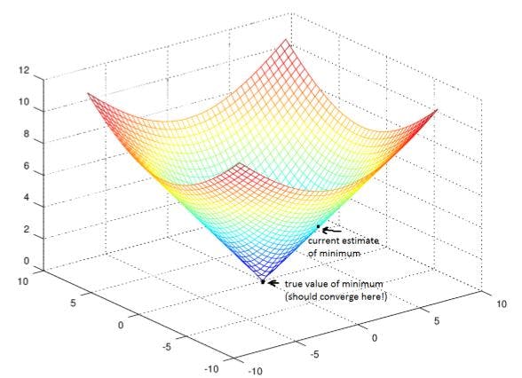
The goal of gradient descent is to find the minimum of our model’s loss function by iteratively getting a better and better approximation of it.

Imagine yourself walking through a valley with a blindfold on. Your goal is to find the bottom of the valley. How would you do it?

A reasonable approach would be to touch the ground around you and move in whichever direction the ground is sloping down most steeply. Take a step and repeat the same process continually until the ground is flat. Then you know you’ve reached the bottom of a valley; if you move in any direction from where you are, you’ll end up at the same elevation or further uphill. Going back to mathematics, the ground becomes our loss function, and the elevation at the bottom of the valley is the minimum of that function.

Now how to look at this mathematically? Now this is a task which we are assigning to you. Go down to the resource section of this post and understand the math behind Gradient Descent.

If you have reached till here, well done! Take a break!

Classification: predicting a label

Is this email spam or not? Is that borrower going to repay their loan? Will those users click on the ad or not? Who is that person in your Facebook picture?

Classification predicts a discrete target label Y . Classification is the problem of assigning new observations to the class to which they most likely belong, based on a classification model built from labeled training data.

Logistic Regression: 0 or 1?

It is a method of classification: the model outputs the probability of a categorical target variable Y belonging to a certain class.

A good example of classification is determining whether a loan application is fraudulent.

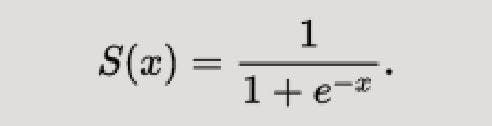
Before moving further let's see what Sigmoid function is:

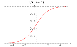
Sigmoid Function squashes the values between 0 and 1.

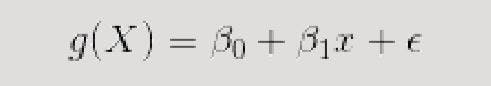
So let's convert g(x) from Linear Regression to a Sigmoid Function.

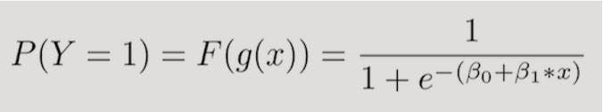
In other words, we’re calculating the probability that the training example belongs to a certain class: P(Y=1).

The output of the logistic regression model from above looks like an S-curve showing P(Y=1) based on the value of X:

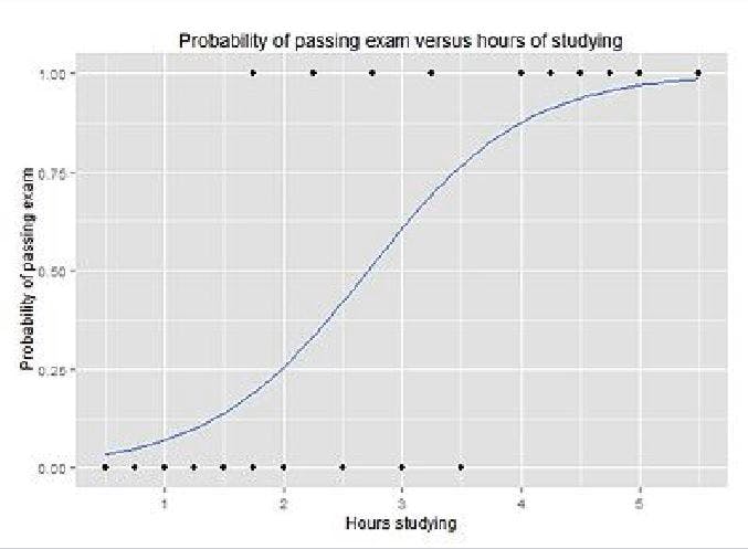
To predict the Y label — spam/not spam, cancer/not cancer, fraud/not fraud, etc. — you have to set a probability cutoff, or threshold, for a positive result. For example: “If our model thinks the probability of this email being spam is higher than 70%, label it spam. Otherwise, don’t."

Minimizing loss with logistic regression

As in the case of linear regression, we use gradient descent to learn the beta parameters that minimize loss.

In logistic regression, the cost function is basically a measure of how often you predicted 1 when the true answer was 0, or vice versa. Below is a regularized cost function just like the one we went over for linear regression.

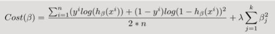
Don't panic yet! Let's break this equation into chunks and see it individually.

1. The first chunk is the data loss, i.e. how much discrepancy there is between the model’s predictions and reality.

2. The second chunk is the regularization loss, i.e. how much we penalize the model for having large parameters that heavily weight certain features.

That's it for Logistic regression.

If you've reached till here, take a small break and continue!

k-nearest neighbors (k-NN)

k-NN seems almost too simple to be a machine learning algorithm. The idea is to label a test data point x by finding the mean (or mode) of the k closest data points’ labels.

Take a look at the image below. Let’s say you want to figure out whether Mysterious Green Circle is a Red Triangle or a Blue Square. What do you do?

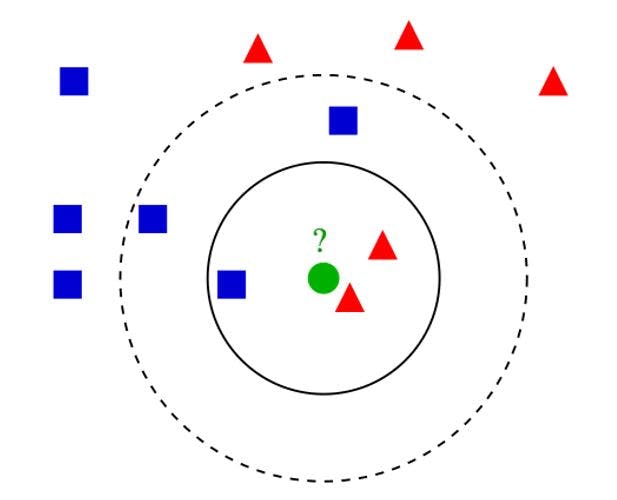
It's simple. You look at the k closest data points and take the average of their values if variables are continuous (like housing prices), or the mode if they’re categorical (like cat vs. dog).

The fact that k-NN doesn’t require a pre-defined parametric function f(X) relating Y to X makes it well-suited for situations where the relationship is too complex to be expressed with a simple linear model.

Now we need to calculate the nearest neighbors. The most straightforward measure is Euclidean distance.

Euclidean distance d(p,q) between points p and q in n-dimensional space:

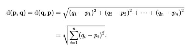
Formula for Euclidean distance, derived from the Pythagorean theorem. With this formula, you can calculate the nearness of all the training data points to the data point you’re trying to label, and take the mean/mode of the k nearest neighbors to make your prediction.

Now we'll move on to Unsupervised Learning.

2. Unsupervised Learning

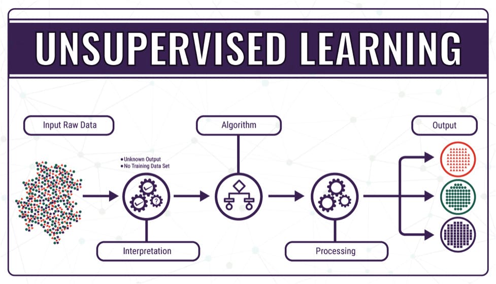
Examples of where unsupervised learning methods might be useful:

• An advertising platform segments the U.S. population into smaller groups with similar demographics and purchasing habits so that advertisers can reach their target market with relevant ads.
• Airbnb groups its housing listings into neighborhoods so that users can navigate listings more easily.
• A data science team reduces the number of dimensions in a large data set to simplify modeling and reduce file size.

k-means clustering

The goal of clustering is to create groups of data points such that points in different clusters are dissimilar while points within a cluster are similar.

With k-means clustering, we want to cluster our data points into k groups. A larger k creates smaller groups with more granularity, a lower k means larger groups and less granularity.

The output of the algorithm would be a set of “labels” assigning each data point to one of the k groups. In k-means clustering, the way these groups are defined is by creating a centroid for each group.

Think of these as the people who show up at a party and soon become the centers of attention because they’re so magnetic. If there’s just one of them, everyone will gather around; if there are lots, many smaller centers of activity will form.

Here are the steps to k-means clustering:

1. Define the k centroids. Initialize these at random (there are also fancier algorithms for initializing the centroids that end up converging more effectively).

2. Find the closest centroid & update cluster assignments. Assign each data point to one of the k clusters. Each data point is assigned to the nearest centroid’s cluster. Here, the measure of “nearness” is a hyperparameter — often Euclidean distance.

3. Move the centroids to the center of their clusters. The new position of each centroid is calculated as the average position of all the points in its cluster.

Keep repeating steps 2 and 3 until the centroid stop moving a lot at each iteration (i.e., until the algorithm converges)

Check out this visualization of the algorithm, you'll understand it more clearly.

Hierarchical clustering

Hierarchical clustering is similar to regular clustering, except that you’re aiming to build a hierarchy of clusters. This can be useful when you want flexibility in how many clusters you ultimately want.

For example, imagine grouping items on an online marketplace like Amazon. On the homepage you’d want a few broad categories of items for simple navigation, but as you go into more specific shopping categories you’d want increasing levels of granularity, i.e. more distinct clusters of items.

Here are the steps for hierarchical clustering:

1. Start with N clusters, one for each data point.
2. Merge the two clusters that are closest to each other. Now you have N-1 clusters.
3. Recompute the distances between the clusters. There are several ways to do this (see this tutorial for more details). One of them (called average-linkage clustering) is to consider the distance between two clusters to be the average distance between all their respective members.
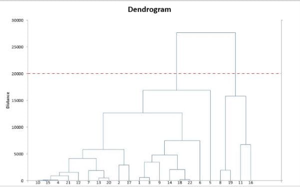
4. Repeat steps 2 and 3 until you get one cluster of N data points. You get a tree (also known as a dendrogram) like the one below.
5. Pick a number of clusters and draw a horizontal line in the dendrogram. For example, if you want k=2 clusters, you should draw a horizontal line around “distance=20000.” You’ll get one cluster with data points 8, 9, 11, 16 and one cluster with the rest of the data points. In general, the number of clusters you get is the number of intersection points of your horizontal line with the vertical lines in the dendrogram.

We'll that's it for now about Unsupervised Learning. Hope you got a detailed overview about Supervised and Unsupervised Learning.

Resources

1. Machine Learning for Humans: We covered a lot of content from here because this is by far the best post we've seen about Supervised and Unsupervised Learning.
2. Machine Learning 101: An Intuitive Introduction to Gradient Descent
3. Understanding the Mathematics behind Gradient Descent

This blog is written by Joel Johnson. Feel free to comment on this post if you have any queries and show us some love by liking the post!

Our next blog will be about Data Preprocessing (for ML in Python). So grab your machine and let's start coding in the next session!